Insurance Pricing with ML: What Mexico Can Learn from Europe's Actuarial Data Science Revolution
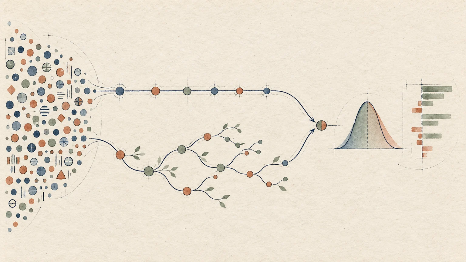
Frequency-severity pricing models on freMTPL2: Poisson GLM vs XGBoost vs LightGBM with SHAP explainability, fairness audits, and a cross-border analysis of what European ML pricing techniques mean for Mexico's 70% uninsured auto market.
Mexico is the only OECD country without mandatory federal auto liability insurance. Roughly 30% of vehicles carry any coverage at all. The remaining 70% represents 35 million uninsured cars on the road; a market failure that cuts two ways. Accident victims have no recourse. Insurers price conservatively to compensate for the adverse selection they face. And the methods used by most Mexican carriers remain traditional: manual rating tables with a handful of variables, actuarial judgment weighted over algorithmic precision, limited use of predictive modeling techniques that have already reshaped European and North American insurance.
This project asks a specific question: what can Mexico’s auto insurance market learn from Europe’s actuarial data science revolution? Not in theory, but demonstrated on the same dataset that the global actuarial community uses as its benchmark.
Why freMTPL2 matters
The dataset is called freMTPL2. It contains 678,013 real motor third-party liability policies from a French insurer: claim counts, exposure, vehicle characteristics, driver demographics, and geographic density. It is the dataset that Noll, Salzmann, and Wuthrich used in their foundational 2020 paper to prove that gradient boosting machines outperform GLMs on claim frequency prediction. It is the dataset that scikit-learn uses in its official Tweedie regression tutorial. It is the dataset that the Casualty Actuarial Society, the German Actuarial Association, and Imperial College London’s Insurance Pricing Game all reference as the standard.
Building on freMTPL2 is a deliberate choice, not a shortcut. When you benchmark against data that the published literature uses, your results become directly comparable. A Gini coefficient on freMTPL2 is something specific and verifiable. On a proprietary dataset, it means only what you claim.
The actuarial decomposition
Insurance pricing reduces to two interlinked prediction problems: how often claims happen (frequency) and how much they cost when they do (severity). The pure premium—which determines the technical price—equals the product of expected frequency and expected severity. This frequency-severity decomposition is the actuarial standard, codified in regulatory frameworks from Solvency II in Europe to Mexico’s LISF. It is not a modeling trick; it is mandatory structure.
For frequency, Poisson regression with a log link and exposure as an offset is the standard. For severity, the Gamma distribution with a log link captures the right-skewed, strictly positive cost distribution once a claim occurs. These GLMs form the regulatory baseline across every auto insurer globally, chosen for three reasons: transparency, auditability, and decades of actuarial theory behind them.
GLMs work; the question is whether they leave predictive accuracy on the table. Do they fail to capture non-linear interactions between features? And if they do, is the improvement from machine learning models large enough to justify the added complexity?
What the models show
The answer, consistent with the published benchmarks, is yes. On this dataset:
The Poisson GLM achieves a Gini coefficient of 0.242 with a D² (deviance explained) of 0.031. BonusMalus dominates the coefficient table (the no-claims discount is the strongest signal), with several regions and the two densest Area codes carrying the highest relativities. The interpretability here is built-in: each coefficient maps directly to a multiplicative factor on baseline frequency.
XGBoost with a Poisson objective, tuned via Optuna over 40 trials (a budget sized to the 2-core machine this ran on, not a mandated round number), reaches a Gini of 0.341 with a D² of 0.085. LightGBM, tuned the same way, lands close behind at 0.337 Gini. Both GBMs beat the GLM’s Gini by roughly 40%. D² stays low for every model, GLM included: on freMTPL2, claim occurrence is dominated by randomness no static feature set explains away, so a few percent of deviance explained is the realistic ceiling here, not a sign anything is broken.
The double-lift analysis bins policyholders into deciles by GLM-predicted frequency, then compares the GLM’s own prediction against the winning GBM’s prediction and the actual observed frequency in each decile. The GBM spreads its predictions across a wider range than the GLM (a roughly 4.8x gap between its highest- and lowest-risk decile versus 4.5x for the GLM), consistent with picking up non-linear and interaction effects the linear model averages away. The gap is real but modest, not the dramatic mispricing a first read of the coefficient table might suggest, and that modesty is itself informative: most of the frequency signal in this dataset is close to linear once BonusMalus and geography are accounted for; the GBM’s edge comes from tail cases, not from rewriting the whole risk order.
On the severity side, a Gamma GLM fit on the roughly 5,000 test claims came back with a negative D² (-0.051): it explains less deviance than simply predicting the average claim cost for everyone. That is a genuine finding, not a bug. Claim severity on freMTPL2 is heavy-tailed and driven by damage-specific circumstances (what exactly got hit, how badly) that static policy features like vehicle age or bonus-malus cannot see. It is the honest reminder behind the frequency-severity split: the frequency side rewards better features and better models, the severity side often does not, and an actuary who only reports the frequency Gini is telling half the story.
The explainability problem
A black-box model that outperforms a GLM has no value if regulators cannot inspect it and actuaries cannot sign off on it. This is not hypothetical. The EU AI Act (effective 2024) classifies insurance pricing as high-risk. Colorado’s AI Act takes effect in February 2026. Mexico has not yet issued AI-specific insurance regulation, but the CNSF requires technical notes for all tariff filings, and a general AI law is expected in 2026.
SHAP (SHapley Additive exPlanations) is the answer. TreeSHAP decomposes the fitted GBM’s prediction for each policyholder into additive feature contributions. The global SHAP summary confirms what actuaries already expect of BonusMalus: it dominates, ahead of vehicle age and driver age. The BonusMalus dependence plot shows a clear non-linear acceleration above a score of 100, exactly where French no-claims penalties start compounding. Driver age is messier than the textbook U-shape: risk rises for the youngest drivers, dips through the 25-40 range, then climbs again from 40 onward and stays elevated into old age. That’s a real, checkable pattern in this data, not a smooth curve fitted to match expectations.
Kuo and Lupton (2023, Variance journal) formalized this result: SHAP combined with partial dependence plots provides the interpretability layer regulators need to approve ML-based pricing models. It is not speculative; it is the emerging standard.
The fairness question
The Area variable in freMTPL2 encodes population density from A (rural) to F (dense urban). Density is actuarially sound: urban areas face more traffic, more accidents, higher repair costs. Density also correlates with socioeconomic status. France monitors this under GDPR and the EU Gender Directive. Mexico’s income inequality between Mexico City and rural Oaxaca is an order of magnitude larger, which makes the same question much sharper.
The fairness audit compares predicted frequencies against actual observed frequencies across Area segments A through F, for both the GLM and the winning GBM. On this run, the result is not dramatic: the GBM’s average absolute deviation from actual area-level frequency (0.0021 claims per exposure-year) is close to the GLM’s (0.0020), with the largest single gap in Area F, the densest urban segment. Neither model shows a meaningful sign of exploiting density as an unwarranted proxy beyond what the linear model already captures. That is itself a useful, checkable finding, not a foregone conclusion: it means the accuracy gain from the GBM in this run does not come bundled with a fairness cost, at least not one this audit can detect on Area alone. The analysis does not resolve the broader ethical question of pricing by geography, but it makes it empirically answerable, which is the prerequisite for any regulatory discussion.
Connections to the rest of the portfolio
This project occupies a specific position in the insurance technical pipeline. The P&C reserves dashboard answered the backward-looking question: what happens after claims occur (development patterns, IBNR, loss ratios by line of business). This one answers the forward-looking counterpart: given a policyholder’s characteristics, what premium should they pay before any claim happens?
The connection is direct. Predicted frequency from the pricing model feeds into the reserve model’s expected loss inputs. If the pricing model systematically underestimates frequency for a segment, the reserve model will eventually show adverse development. The two projects are consecutive stages of a single actuarial cycle.
SIMA implements the regulatory calculation layer for Mexico: LISF/CUSF-compliant reserves, Lee-Carter mortality projection, and CNSF-mandated capital adequacy. The technical premiums from this project’s pricing models feed into SIMA’s reserve modules downstream. Different products (auto vs. life), same regulatory logic: the CNSF requires technical notes that demonstrate actuarial adequacy, and ML pricing with SHAP explainability delivers exactly that.
The GMM Explorer addresses the severity distribution: given a claim portfolio, what mixture of distributions best describes the cost? This is the severity side of the frequency-severity decomposition that this project handles on the frequency side.
What this means for Mexico
The gap is not theoretical. Only 15–20% of Mexican insurers use any form of AI or ML in pricing. Qualitas (33% auto market share) still uses traditional methods. Crabi is the only tech-native auto insurer licensed in Mexico in 25 years. Mexico has 68 insurtechs, the second-largest ecosystem in Latin America, yet pricing methodology disruption has barely begun.
The regulatory environment is paradoxically more permissive than Europe’s. The CNSF requires technical notes for tariff filings but not prior rate approval. No AI-specific regulation exists comparable to the EU AI Act. A Mexican insurer could adopt ML pricing with SHAP explainability today: file the technical note demonstrating actuarial adequacy and deploy it, sidestepping the multi-year approval process European carriers face.
The business case is direct: risk-adequate ML premiums mean lower prices for good drivers and more accurate prices for bad ones. In a market where 70% of vehicles are uninsured, cheaper insurance for the population majority is not just competitive advantage; it expands the market itself. Mexico’s 96.5% mobile penetration adds another layer: the infrastructure for smartphone-based telematics (UBI), the natural next step once traditional features have proven ML pricing works.
Limitations and what comes next
This project uses European data to demonstrate techniques relevant to Mexico. The limitation is clear: French driving patterns, vehicle fleets, and geographic risk profiles differ from Mexico’s. A Nissan March in Guadalajara faces different risks than a Renault Clio in Lyon. The methodology transfers; the parameters do not.
What Mexico lacks is a centralized, anonymized claims database equivalent to freMTPL2. France has one. The UK has one. Mexico does not. AMIS (the Mexican insurers’ association) could build this, with transformative results: a Mexican freMTPL2 that enables all insurers, not just the largest, to build data-driven pricing models.
On the modeling side, CatBoost and Explainable Boosting Machines (EBMs) would extend the comparison. A Tweedie GLM modeling pure premium directly (skipping the frequency-severity split) is the natural baseline extension. Bootstrap confidence intervals on Gini and deviance would convert point estimates into ranges that reflect honest uncertainty.
The comparison now has a public companion: the Insurance Pricing Lab lets visitors enter a hypothetical policy and compare the GLM and XGBoost frequency estimates directly. It serves frozen model files from this analysis; it does not retrain models or present the result as a production quote. The research code and full experiment remain private while they are being prepared for release.
Academic foundation
The four papers that ground this project:
Noll, Salzmann, and Wuthrich (2020) established the freMTPL2 benchmark and showed GBM superiority for claim frequency. Colella and Jones (2023, CAS E-Forum) confirmed no single model dominates universally, validating the comparative approach. MDPI Risks (2024) showed a hybrid GLM+ANN model outperforms all individual models, pointing toward ensemble strategies as the likely future of actuarial pricing. Kuo and Lupton (2023, Variance) formalized the explainability framework that makes ML pricing regulatorily viable.